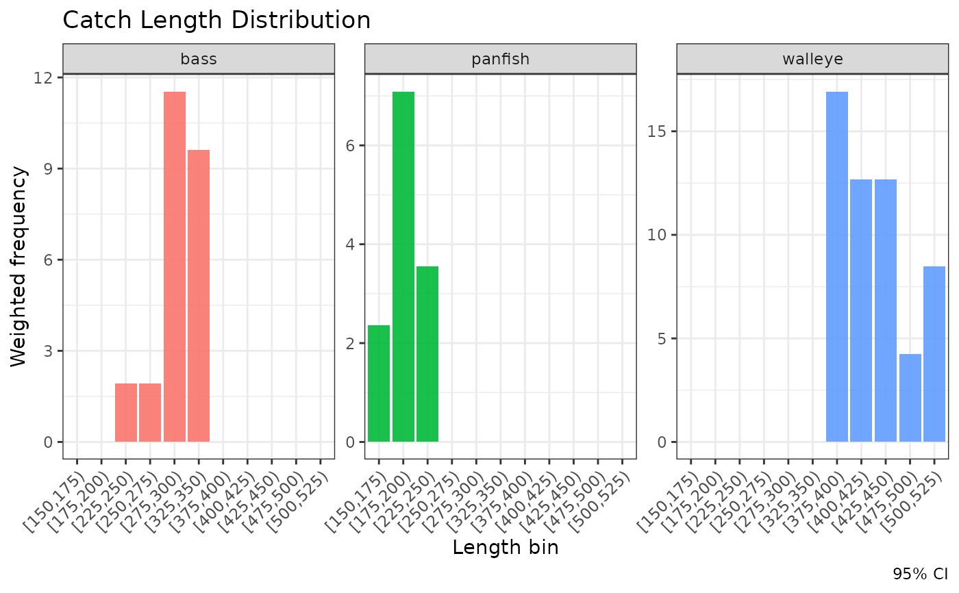
Plot a weighted length distribution with ggplot2

autoplot.creel_length_distribution() renders weighted length-frequency estimates as a histogram-style bar chart. Ungrouped results are shown as a single distribution; grouped results are faceted by the grouping variables.

Usage

# S3 method for class 'creel_length_distribution'
autoplot(object, title = NULL, theme = c("default", "creel"), ...)

Arguments

object

A creel_length_distribution object returned by est_length_distribution().

title

Optional plot title. Defaults to a title derived from the estimated fish type (catch, harvest, or release).

theme

Character string selecting the plot theme. Use "default" (default) for ggplot2::theme_bw(), or "creel" for theme_creel() and package-standard colours. Neither inherits a theme set with ggplot2::theme_set(); add your own with + if you need it.

...

Additional arguments (currently unused).

Value

A ggplot object.

See also

est_length_distribution()

Other "Visualisation": autoplot.creel_estimates(), autoplot.creel_schedule(), creel_palette(), plot_design(), theme_creel()

Examples

data(example_calendar)
data(example_interviews)
data(example_catch)
data(example_lengths)

design <- creel_design(example_calendar, date = date, strata = day_type)
design <- add_interviews(design, example_interviews,
  catch = catch_total, effort = hours_fished, harvest = catch_kept,
  trip_status = trip_status
)
#> Warning: ! No `n_anglers` provided — assuming 1 angler per interview.
#> ℹ Pass `n_anglers = <column>` to use actual party sizes for angler-hour
#>   normalization.
#> ℹ If the interviews really are one angler each, pass `n_anglers = 1` to state
#>   that and silence this warning.
#> ℹ Added 22 interviews: 17 complete (77%), 5 incomplete (23%)
# Species catch is required to group by species: length totals are scaled
# onto the reported catch, and only this table records it per species.
design <- add_catch(design, example_catch,
  catch_uid = interview_id, interview_uid = interview_id,
  species = species, count = count, catch_type = catch_type
)
design <- add_lengths(design, example_lengths,
  length_uid = interview_id, interview_uid = interview_id,
  species = species, length = length, length_type = length_type,
  count = count, release_format = "binned"
)

ld <- est_length_distribution(design, by = species, bin_width = 25)
#> Warning: ! Length totals were rescaled onto the reported catch.
#> ℹ Measured fish (weighted): 37; reported: 93 -- a factor of 2.51.
#> ℹ estimate, se and the confidence bounds describe the REPORTED catch, estimated
#>   from the measured subsample. Shares (percent) are unaffected.
ggplot2::autoplot(ld)