Survey Design Toolbox: Planning, Comparing, and Combining Designs

This vignette collects three M014 tools into one practitioner-facing workflow:

power_creel() for pre-season sample-size and power planning
compare_designs() for side-by-side comparison of completed survey estimates
as_hybrid_svydesign() for combining disjoint count frames in a single survey design

library(tidycreel)

1 Pre-season sample-size planning with `power_creel()`

Pre-season planning usually starts with pilot information: expected effort by stratum, variability in daily counts, and rough interview-level CV values for catch and effort. power_creel() provides one interface for three planning questions.

Required sampling days for total effort precision

This first example estimates how many sampling days are needed in weekday and weekend strata to target a 20% RSE on the seasonal effort estimate.

effort_plan <- power_creel(
  mode = "effort_n",
  target_rse = 0.20,
  strata = c("weekday", "weekend"),
  N_h = c(90, 30),
  ybar_h = c(42, 68),
  s2_h = c(196, 441)
)

effort_plan
#>     stratum n_required target_rse
#> 1   weekday          3        0.2
#> 2   weekend          1        0.2
#> 3     total          3        0.2
#> 4 allocated          4        0.2

The result returns one row per stratum plus a total row, making it easy to translate a seasonal precision target into a day-allocation plan.

Required interviews for CPUE precision

If the planning question is interview effort rather than count days, mode = "cpue_n" solves for the number of interviews needed to estimate CPUE with a target RSE.

cpue_plan <- power_creel(
  mode = "cpue_n",
  target_rse = 0.15,
  cv_catch = 0.85,
  cv_effort = 0.55,
  rho = 0.35
)

cpue_plan
#>   n_required target_rse cv_catch cv_effort  rho
#> 1         32       0.15     0.85      0.55 0.35

This is useful when interview staffing is the main operational bottleneck and pilot data already suggest the variability of catch and angler effort.

Power to detect a management-relevant CPUE change

The third mode asks a different question: if we can complete a fixed number of interviews, how much power do we have to detect a change in CPUE from one season to the next?

power_plan <- power_creel(
  mode = "power",
  n = 120L,
  cv_historical = 0.42,
  delta_pct = 0.20
)

power_plan
#>       power   n delta_pct cv_historical alpha alternative
#> 1 0.9580589 120       0.2          0.42  0.05   two.sided

Here delta_pct = 0.20 means a 20% change in CPUE. Together, the three modes cover the most common pre-season planning decisions: how many days to sample, how many interviews to complete, and what power that design can deliver.

2 Comparing finished designs with `compare_designs()`

Once a survey has been completed, compare_designs() helps compare multiple creel_estimates objects on a common scale. In this example we estimate total effort twice from the same dataset, changing only the variance method.

data("example_counts")
data("example_interviews")

calendar <- unique(example_counts[, c("date", "day_type")])

design <- creel_design(calendar, date = date, strata = day_type)
design <- add_counts(design, example_counts)
design <- add_interviews(
  design,
  example_interviews,
  catch = catch_total,
  effort = hours_fished,
  trip_status = trip_status,
  n_anglers = n_anglers
)

set.seed(123)

effort_taylor <- estimate_effort(design, variance = "taylor")
effort_bootstrap <- estimate_effort(design, variance = "bootstrap")

design_comparison <- compare_designs(
  list(
    Taylor = effort_taylor,
    Bootstrap = effort_bootstrap
  )
)

design_comparison
#> 
#> ── Survey Design Comparison ────────────────────────────────────────────────────
#> 2 row(s), 2 design(s)
#> 
#>      design estimate   se    rse ci_lower ci_upper ci_width  n
#> 1    Taylor      372 13.2 0.0354      344      401     57.4 14
#> 2 Bootstrap      372 13.5 0.0363      343      402     58.9 14

Because both estimates come from the same counts and interviews, the point estimate is identical while the uncertainty metrics reflect the different variance estimators.

ggplot2::autoplot(design_comparison)
#> `height` was translated to `width`.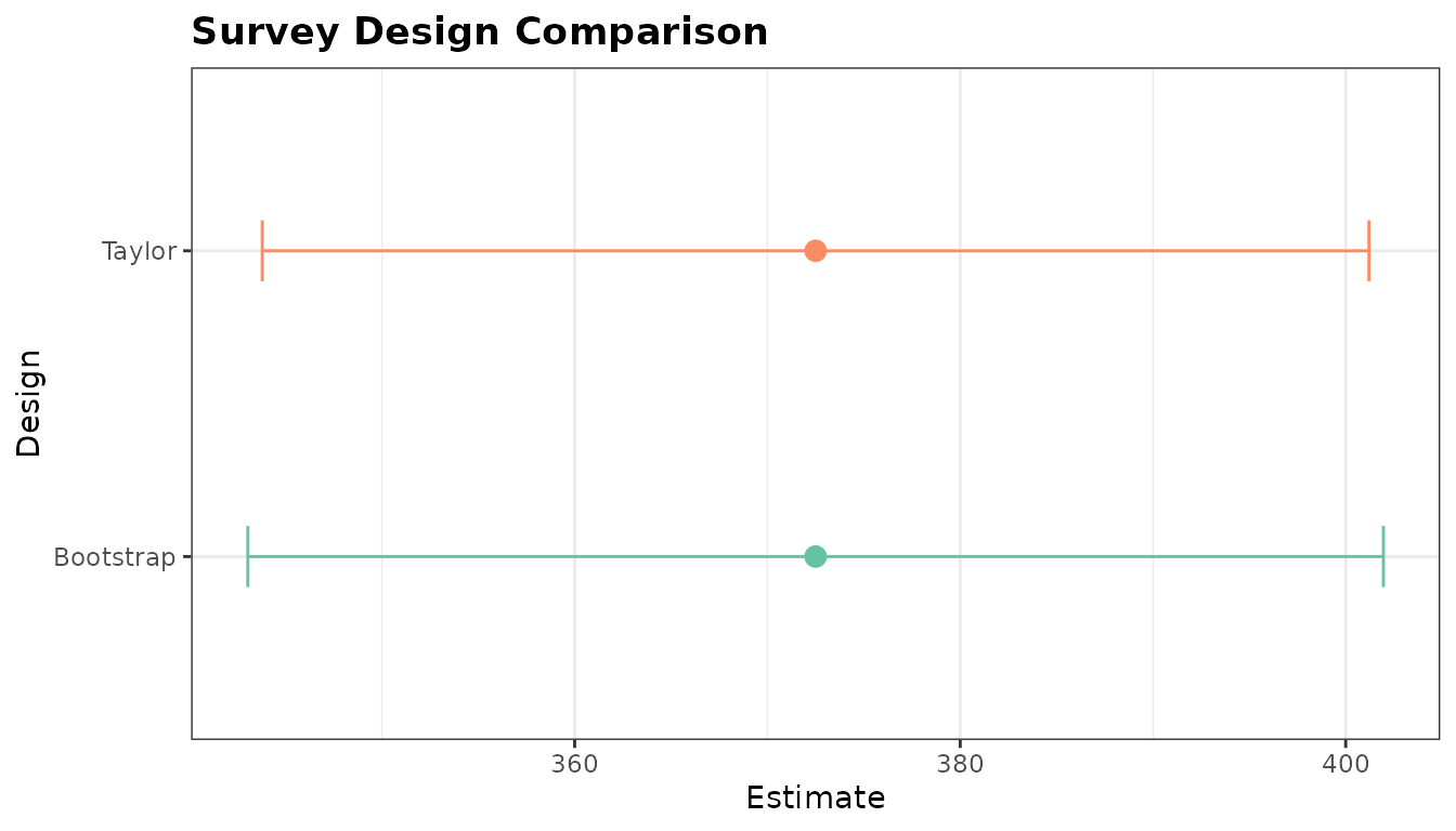

Design comparison across two effort estimators.

This pattern is helpful after a season when you want to compare alternative estimation choices without rebuilding custom summary tables by hand.

3 Combining disjoint count frames with `as_hybrid_svydesign()`

Some programs count disjoint parts of a fishery separately — most often boat anglers and bank anglers, which are reached by different field methods and enumerated at different rates. as_hybrid_svydesign() combines those count series into a single survey design object, treating each as its own stratum with its own within-day sampling fraction, and clustering observations on the date so the date is the primary sampling unit.

A note on the vocabulary. In the creel literature access and roving describe how anglers are interviewed — access interviews intercept completed trips as anglers leave, roving interviews intercept incomplete trips while they fish — and a survey mixing the two is a hybrid interview design. Counts are not described that way; they are instantaneous, progressive, bus-route, camera or aerial. tidycreel carries the interview axis on add_interviews()’s interview_type argument. What this function takes is a count frame: a disjoint part of the fishery with its own count, typically an angler-type domain such as boat or bank anglers. You name the column holding that partition with frame_col, and its values become the frame labels — so the design speaks your vocabulary rather than borrowing the interview one.

The design estimates a period total — the total over every day in the season, not over the days that happened to be sampled. Two expansions get it there, and both live in the row weight. The within-day fraction expands the part of a frame that the count enumerated to the whole of it. N_h / n_h expands the sampled days to the days the stratum holds, which is why a calendar is required: the sampled dates alone cannot say how long a stratum is. Only the second of the two is a sampling fraction over the date PSUs, so only the second drives the finite-population correction.

Every frame shares the calendar. One stratum is one span of the season, whichever frame observed it.

Adding the frame totals is valid only when the frames sample disjoint sets of angler trips — no angler trip may be observed by more than one. That is a property of the field protocol, not of the data, so tidycreel cannot check it and asks you to affirm it with trips_disjoint = TRUE.

Each frame may contribute at most one count row per date. Two counts on a date are two looks at that date, not two sampled days, and a per-day expansion is undefined for them; average them to one row per date first.

calendar <- data.frame(
  date = seq(as.Date("2024-06-01"), as.Date("2024-06-30"), by = "day")
)
calendar$day_type <- ifelse(
  format(calendar$date, "%u") %in% c("6", "7"), "weekend", "weekday"
)

counts <- data.frame(
  date = rep(
    as.Date(c("2024-06-03", "2024-06-08", "2024-06-10", "2024-06-15")),
    times = 2
  ),
  day_type = rep(c("weekday", "weekend", "weekday", "weekend"), times = 2),
  angler_type = rep(c("boat", "bank"), each = 4),
  count = c(12L, 18L, 9L, 21L, 10L, 16L, 8L, 19L)
)

hybrid_design <- as_hybrid_svydesign(
  counts,
  frame_col = "angler_type",
  calendar = calendar,
  fraction = list(
    boat = c(weekday = 0.5, weekend = 0.5),
    bank = c(weekday = 0.5, weekend = 0.5)
  ),
  trips_disjoint = TRUE
)

hybrid_design
#> 
#> ── Hybrid Creel Survey Design ──────────────────────────────────────────────────
#> Frames: bank (4 obs) and boat (4 obs)
#> 
#> Stratified Independent Sampling design
#> survey::svydesign(ids = ids_formula, strata = strata_formula, 
#>     weights = weights_formula, fpc = ~.pop_days, data = combined, 
#>     nest = TRUE)

The returned object is a survey design rather than a creel_design, so estimate_effort() does not accept it; estimate from it with survey directly.

survey::svytotal(~count, hybrid_design)
#>       total    SE
#> count  1520 78.23

That total is a season total: 20 weekday days and 10 weekend days in the June calendar, expanded from the two of each that were sampled.

This small example is intentionally self-contained, but the same pattern scales to real field programs where the count frames cover complementary, non-overlapping parts of the fishery, and to more than two of them. Every frame should sample the same days — the function warns when their date-stratum coverage is asymmetric — while covering different anglers or different water is exactly what makes their totals addable.

Summary

The survey-design toolbox supports the full planning-to-reporting arc:

power_creel() helps set realistic pre-season sample sizes and power targets
compare_designs() turns alternative estimator outputs into a tidy, directly comparable object with a plotting method
as_hybrid_svydesign() bridges programs that count two disjoint parts of a fishery separately into one survey design for downstream analysis

Used together, these tools make it easier to justify sampling effort before the season, evaluate estimator trade-offs afterward, and support hybrid monitoring programs with standard survey workflows.

1 Pre-season sample-size planning with power_creel()