Bus-Route Surveys • tidycreel

What is a Bus-Route Survey?

A bus-route survey visits multiple access points (sites) in a fixed route, called a circuit. Unlike an access-point creel survey that stations an interviewer at one location for the day, a bus-route crew travels the circuit repeatedly, counting and interviewing anglers at each site as they pass through.

Sites are not weighted equally. The crew visits every site on each pass but waits longer at busier sites (Jones & Pollock 2012, Box 19.3), so a party at a busy site is more likely to be seen. A site’s weight is the share of the circuit the crew spends there: its wait divided by the time to complete the whole circuit, travel included (Robson & Jones 1989; Pollock et al. 1994, eq. 15.10). Inverse weighting by that share is what makes the estimate unbiased.

Two types of data are collected during each visit:

Enumeration counts — every angler party at the site is counted (n_counted).
Interviews — a subset of parties is interviewed to collect effort and catch data (n_interviewed).

The ratio n_counted / n_interviewed (the enumeration expansion factor) scales the interviewed catch and effort up to represent all parties at the site, including those not interviewed. Without this expansion, busy sites are systematically underrepresented in the total estimate.

The estimator is the bus-route design of Robson & Jones (1989), as set out in Pollock et al. (1994, section 15.5.3). It is written in the general Horvitz-Thompson form of Jones & Pollock (2012, Chapter 19).

Key Concepts

Inclusion Probability (πᵢ)

The inclusion probability πᵢ is the probability that a given sampling unit (site × period combination) is included in the sample. For a two-stage bus-route design:

$\pi_i = p\_site_i \times p\_period$

where p_period is the probability that the period containing the visit is sampled, and p_site is the site’s weight within the circuit. It can be given in two ways:

wait_time and circuit_time, for a route that visits every site on each pass. p_site is then wait_time / circuit_time. These shares add up to less than 1 whenever the route has travel time, and that is correct: no party can be seen while the crew is driving.
p_site, the probability that a pass selects the site, for a design in which each pass visits a randomly chosen site. These probabilities add up to 1 within a circuit.

Do not rescale wait times so that they add up to 1. That divides by the total wait rather than the circuit time, and every total comes out too low by the share of the circuit spent travelling.

The inclusion probability πᵢ belongs to the sampling design, not to a site or its anglers. Specify it when designing the survey; do not compute it from the interview data.

Enumeration Counts

During each circuit pass, the crew counts every visible angler party at the site (n_counted) and then interviews as many as possible (n_interviewed). When not all parties are interviewed, the expansion factor

$\text{expansion} = \frac{n\_counted}{n\_interviewed}$

rescales the interviewed data so it represents all parties. If all parties are interviewed (n_counted = n_interviewed), the expansion is 1 and no adjustment is needed, as in the example below.

Horvitz-Thompson Estimator

The total effort estimator (Jones & Pollock 2012, Eq. 19.4) is:

$\hat{E} = \sum_i \frac{e_i}{\pi_i}$

where $e_i = \text{hours\_fished}_i \times \text{expansion}_i$ is the enumeration-expanded effort for interview i. Each site’s contribution is weighted by the reciprocal of its inclusion probability. A site sampled with probability 0.20 receives weight 5 — five times the weight of a site sampled with probability 1.0. This inverse-probability weighting is what makes the estimator statistically unbiased.

The harvest estimator (Jones & Pollock 2012, Eq. 19.5) follows the same structure:

$\hat{H} = \sum_i \frac{h_i}{\pi_i}$

Choosing the Site Weights

Some implementations fix $\pi_i = 0.5$ for every site. That is not an inclusion probability of the design, and each site’s contribution is then off by the ratio of 0.5 to its true $\pi_i$ .

tidycreel computes $\pi_i = p\_site \times p\_period$ from the sampling frame you give creel_design(), with p_site either supplied directly or computed as wait_time / circuit_time. The test suite reproduces the bus-route effort and catch examples in Pollock et al. (1994, Tables 15.16 and 15.17) from wait and circuit times. Malvestuto (1996, Box 20.6) uses the same inverse-probability rule in its access-point and roving examples, and the test suite reproduces its Examples 1 and 2.

Step-by-Step Example

We demonstrate the full bus-route workflow on a small constructed example: a four-site, single-circuit survey with 15 interviews over four days. The numbers are invented, so the totals below are this example’s own arithmetic, not published figures. The test suite checks the same estimator against a published example, Pollock et al. (1994, Tables 15.16 and 15.17); the equations page works through it.

Step 1: Define the Sampling Design

The sampling frame lists the four sites, the crew’s scheduled wait at each, and the time to drive the whole circuit once, waits included: 400 minutes, of which 200 are waits and 200 are travel. Each day the crew works either the morning or the afternoon, chosen with equal probability, so p_period = 0.5.

library(tidycreel)

# Sampling frame: 4 sites, 1 circuit. Waits are longer at busier sites.
sampling_frame <- data.frame(
  site        = c("A", "B", "C", "D"),
  circuit     = "circ1",
  wait_min    = c(60, 50, 80, 10), # 200 min of waits
  circuit_min = 400, # whole circuit, travel included
  p_period    = 0.50 # morning or afternoon, equally likely
)
# Site weight: p_site = wait / circuit time; pi_i = p_site * p_period
# Site A: 60 / 400 = 0.150; x 0.5 = 0.0750
# Site B: 50 / 400 = 0.125; x 0.5 = 0.0625
# Site C: 80 / 400 = 0.200; x 0.5 = 0.1000
# Site D: 10 / 400 = 0.025; x 0.5 = 0.0125

# Survey calendar: 4 weekdays
calendar <- data.frame(
  date     = as.Date(c("2024-06-01", "2024-06-02", "2024-06-03", "2024-06-04")),
  day_type = "weekday"
)

# Build the bus-route design
design <- creel_design(
  calendar,
  date = date,
  strata = day_type,
  survey_type = "bus_route",
  sampling_frame = sampling_frame,
  site = site,
  circuit = circuit,
  wait_time = wait_min,
  circuit_time = circuit_min,
  p_period = p_period
)
print(design)
#> 
#> ── Creel Survey Design ─────────────────────────────────────────────────────────
#> Type: "bus_route"
#> Date column: date
#> Strata: day_type
#> Calendar: 4 days (2024-06-01 to 2024-06-04)
#> day_type: 1 level
#> Counts: "none"
#> Interviews: "none"
#> Sections: "none"
#> 
#> ── Bus-Route Design ──
#> 
#> Sites: 4, Circuits: 1
#> Sampling probabilities (pi_i = p_site * p_period):
#> A [circ1]: p_site=0.15, p_period=0.5, pi_i=0.075
#> B [circ1]: p_site=0.125, p_period=0.5, pi_i=0.0625
#> C [circ1]: p_site=0.2, p_period=0.5, pi_i=0.1
#> D [circ1]: p_site=0.025, p_period=0.5, pi_i=0.0125

The design object stores the sampling frame and precomputes πᵢ for each site×circuit combination. The four site shares add up to 0.5, not 1: half the circuit is spent driving, when no party can be seen. Site C has the longest wait and therefore the highest πᵢ (0.10), so each of its parties stands for fewer unseen ones than a party at Site D (πᵢ = 0.0125).

Step 2: Attach Interview Data

Each row of interview data represents one interviewed party. The n_counted and n_interviewed columns record how many parties were at the site vs. how many were actually interviewed. In this example both are equal (no expansion needed), but the columns must still be supplied for bus-route designs.

Each party’s effort is recorded here as angler-hours: the hours fished times the number of anglers in the party. Because the column already counts every angler, n_anglers = 1 tells add_interviews() to take each value as it stands. If your sheet records hours per party and party size separately, pass the hours as effort and the party size as n_anglers instead, and tidycreel multiplies them.

# 15 interviews across 4 sites and 4 days
# Site A: 4 interviews (all 4 parties interviewed)
# Site B: 3 interviews (all 3 parties)
# Site C: 6 interviews (all 6 parties) — highest effort site
# Site D: 2 interviews (all 2 parties)
interviews_raw <- data.frame(
  date = as.Date(c(
    "2024-06-01", "2024-06-01", "2024-06-02", "2024-06-02", # Site A
    "2024-06-01", "2024-06-02", "2024-06-03", # Site B
    "2024-06-01", "2024-06-02", "2024-06-03", # Site C (rows 1-3)
    "2024-06-03", "2024-06-04", # Site C (rows 4-5)
    "2024-06-03", "2024-06-04", # Site D
    "2024-06-03" # Site C (row 6)
  )),
  day_type = "weekday",
  site = c(
    "A", "A", "A", "A",
    "B", "B", "B",
    "C", "C", "C",
    "C", "C",
    "D", "D",
    "C"
  ),
  circuit = "circ1",
  angler_hours = c(
    7.5, 7.5, 7.5, 7.5, # Site A: 4 x 7.5 = 30 h total
    20.0 / 3, 20.0 / 3, 20.0 / 3, # Site B: 3 x 6.67 = 20 h total
    57.5 / 6, 57.5 / 6, 57.5 / 6, # Site C rows 1-3
    57.5 / 6, 57.5 / 6, # Site C rows 4-5
    2.5, 2.5, # Site D: 2 x 2.5 = 5 h total
    57.5 / 6 # Site C row 6: total = 57.5 h
  ),
  fish_kept = c(
    1L, 0L, 1L, 0L,
    1L, 0L, 1L,
    1L, 1L, 0L,
    1L, 0L,
    0L, 0L,
    1L
  ),
  fish_caught = c(
    2L, 1L, 1L, 1L,
    2L, 1L, 1L,
    2L, 1L, 1L,
    1L, 1L,
    1L, 1L,
    1L
  ),
  n_counted = c(
    4L, 4L, 4L, 4L,
    3L, 3L, 3L,
    6L, 6L, 6L,
    6L, 6L,
    2L, 2L,
    6L
  ),
  n_interviewed = c(
    4L, 4L, 4L, 4L,
    3L, 3L, 3L,
    6L, 6L, 6L,
    6L, 6L,
    2L, 2L,
    6L
  ),
  trip_status = "complete"
)

# Attach interviews — pi_i is joined automatically from the sampling frame
design <- add_interviews(
  design,
  interviews_raw,
  effort        = angler_hours,
  catch         = fish_caught,
  harvest       = fish_kept,
  n_counted     = n_counted,
  n_interviewed = n_interviewed,
  trip_status   = trip_status,
  n_anglers     = 1
)
#> ℹ Added 15 interviews: 15 complete (100%), 0 incomplete (0%)
print(design)
#> 
#> ── Creel Survey Design ─────────────────────────────────────────────────────────
#> Type: "bus_route"
#> Date column: date
#> Strata: day_type
#> Calendar: 4 days (2024-06-01 to 2024-06-04)
#> day_type: 1 level
#> Counts: "none"
#> Interviews: 15 observations
#> Type: "access"
#> Catch: fish_caught
#> Effort: angler_hours
#> Harvest: fish_kept
#> Trip status: 15 complete, 0 incomplete
#> Survey: <survey.design2> (constructed)
#> Sections: "none"
#> 
#> ── Bus-Route Design ──
#> 
#> Sites: 4, Circuits: 1
#> Sampling probabilities (pi_i = p_site * p_period):
#> A [circ1]: p_site=0.15, p_period=0.5, pi_i=0.075
#> B [circ1]: p_site=0.125, p_period=0.5, pi_i=0.0625
#> C [circ1]: p_site=0.2, p_period=0.5, pi_i=0.1
#> D [circ1]: p_site=0.025, p_period=0.5, pi_i=0.0125
#> 
#> ── Enumeration Counts ──
#> 
#> (n_counted observed, n_interviewed interviewed, expansion =
#> n_counted/n_interviewed)
#> A [circ1]: counted=16, interviewed=16, expansion=1
#> B [circ1]: counted=9, interviewed=9, expansion=1
#> C [circ1]: counted=36, interviewed=36, expansion=1
#> D [circ1]: counted=4, interviewed=4, expansion=1

add_interviews() joins πᵢ from the sampling frame to each interview row (stored as .pi_i) and computes the enumeration expansion factor (.expansion = n_counted / n_interviewed). These are used internally by the estimation functions.

Step 3: Estimate Effort

estimate_effort() dispatches to the bus-route estimator and computes $\hat{E} = \sum(e_i / \pi_i)$ .

# Estimate total angler-hours
effort_est <- estimate_effort(design)
print(effort_est)
#> 
#> ── Creel Survey Estimates ──────────────────────────────────────────────────────
#> Method: Total
#> Variance: Taylor linearization
#> Confidence level: 95%
#> Effort target: sampled_days
#> Unit: angler-hours
#> 
#> # A tibble: 1 × 5
#>   estimate    se ci_lower ci_upper     n
#>      <dbl> <dbl>    <dbl>    <dbl> <int>
#> 1     1695  248.    1208.    2182.    15

# Inspect per-site contributions to the total
site_contribs <- get_site_contributions(effort_est)
print(site_contribs)
#> # A tibble: 15 × 5
#>    site  circuit   e_i   pi_i e_i_over_pi_i
#>    <chr> <chr>   <dbl>  <dbl>         <dbl>
#>  1 A     circ1    7.5  0.075          100  
#>  2 A     circ1    7.5  0.075          100  
#>  3 A     circ1    7.5  0.075          100  
#>  4 A     circ1    7.5  0.075          100  
#>  5 B     circ1    6.67 0.0625         107. 
#>  6 B     circ1    6.67 0.0625         107. 
#>  7 B     circ1    6.67 0.0625         107. 
#>  8 C     circ1    9.58 0.1             95.8
#>  9 C     circ1    9.58 0.1             95.8
#> 10 C     circ1    9.58 0.1             95.8
#> 11 C     circ1    9.58 0.1             95.8
#> 12 C     circ1    9.58 0.1             95.8
#> 13 D     circ1    2.5  0.0125         200  
#> 14 D     circ1    2.5  0.0125         200  
#> 15 C     circ1    9.58 0.1             95.8

The site contributions table shows exactly how each site’s effort feeds into the total. Site C (πᵢ = 0.10, observed effort 57.5 h) contributes 57.5 / 0.10 = 575 angler-hours, the largest single-site contribution. Site D (πᵢ = 0.0125, observed effort 5 h) contributes 5 / 0.0125 = 400 angler-hours: the crew waits there for only 10 minutes of each 400, so each party seen stands for many that were not.

The total is over the four sampled days. Bus-route totals refuse target = "stratum_total" and "period_total" (the expansion to unsampled days is not implemented).

Step 4: Estimate Catch and Harvest

estimate_harvest_rate() gives fish kept per angler-hour. The totals apply the same Horvitz-Thompson logic as effort, dividing each party’s fish by its inclusion probability and summing.

# Fish kept per angler-hour
harvest_rate <- estimate_harvest_rate(design)
print(harvest_rate)
#> 
#> ── Creel Survey Estimates ──────────────────────────────────────────────────────
#> Method: Ratio-of-Means HPUE
#> Variance: Taylor linearization
#> Confidence level: 95%
#> Unit: fish/angler-hour
#> 
#> # A tibble: 1 × 5
#>   estimate     se ci_lower ci_upper     n
#>      <dbl>  <dbl>    <dbl>    <dbl> <int>
#> 1   0.0582 0.0160   0.0269   0.0896    15

# Total fish kept (harvest) and total fish caught (kept + released)
harvest_est <- estimate_total_harvest(design)
print(harvest_est)
#> 
#> ── Creel Survey Estimates ──────────────────────────────────────────────────────
#> Method: Total Harvest (Horvitz-Thompson)
#> Variance: Taylor linearization
#> Confidence level: 95%
#> Effort target: sampled_days
#> Unit: fish
#> 
#> # A tibble: 1 × 5
#>   estimate    se ci_lower ci_upper     n
#>      <dbl> <dbl>    <dbl>    <dbl> <int>
#> 1     98.7  35.7     28.8     169.    15

catch_est <- estimate_total_catch(design)
print(catch_est)
#> 
#> ── Creel Survey Estimates ──────────────────────────────────────────────────────
#> Method: Total Catch (Horvitz-Thompson)
#> Variance: Taylor linearization
#> Confidence level: 95%
#> Effort target: sampled_days
#> Unit: fish
#> 
#> # A tibble: 1 × 5
#>   estimate    se ci_lower ci_upper     n
#>      <dbl> <dbl>    <dbl>    <dbl> <int>
#> 1     361.  59.9     243.     478.    15

Step 5: Results as Data

Each estimate converts to a tibble with its method, variance method and unit as columns, ready for dplyr or a report table, and plots with its confidence interval:

tibble::as_tibble(catch_est)
#> # A tibble: 1 × 10
#>   estimate    se ci_lower ci_upper     n method       variance_method conf_level
#>      <dbl> <dbl>    <dbl>    <dbl> <int> <chr>        <chr>                <dbl>
#> 1     361.  59.9     243.     478.    15 ht-total-ca… taylor                0.95
#> # ℹ 2 more variables: effort_target <chr>, unit <chr>

ggplot2::autoplot(catch_est)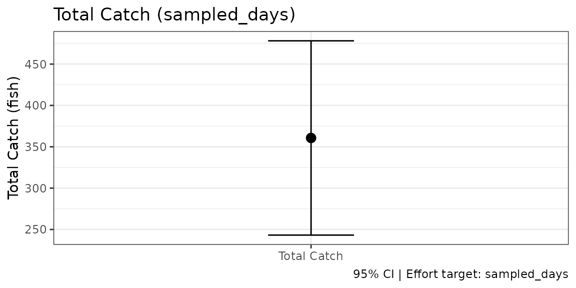

Total catch estimate with its 95 percent confidence interval.

Checking the Arithmetic

Each site contributes its observed effort divided by its inclusion probability:

Site	wait / circuit	πᵢ	e_i (h)	e_i / πᵢ
A	60 / 400	0.0750	30.0	400
B	50 / 400	0.0625	20.0	320
C	80 / 400	0.1000	57.5	575
D	10 / 400	0.0125	5.0	400
Total				1,695

Rescaling the waits to add up to 1 (60/200, 50/200, …) would have given 847.5, half the total, because half the circuit is travel. That is the error the wait_time and circuit_time arguments exist to prevent.

References

Jones, C. M., & Pollock, K. H. (2012). Recreational angler survey methods: estimation of effort, harvest, and released catch. Chapter 19 in Fisheries Techniques (3rd ed.), pp. 883–919. American Fisheries Society.
Malvestuto, S. P. (1996). Sampling the recreational creel. Chapter 20 in Fisheries Techniques (2nd ed.), pp. 591–623. American Fisheries Society.
Pollock, K. H., Jones, C. M., & Brown, T. L. (1994). Angler survey methods and their applications in fisheries management. American Fisheries Society Special Publication 25.
Robson, D., & Jones, C. M. (1989). The theoretical basis of an access site angler survey design. Biometrics, 45, 83–98.