How an Instantaneous Count Becomes Angler-Hours

Estimating fishing effort across sampled days and the full survey period

An instantaneous count measures anglers at one moment. A tidycreel 7.0.0 example shows how period length, survey strata, and sampled days turn those observations into angler-hours with uncertainty.

The previous post kept counts, interviews, catch, and biological observations in linked tables. With those pieces attached to the design, the next question is what they estimate.

Effort comes first. A common mistake among people who are less familiar with creel surveys is to assume that effort comes from interviews because anglers report how long they have fished. In the instantaneous-count design discussed here, those reported hours help estimate catch or harvest per unit effort. They do not provide the total fishing pressure across the survey period.

Counts provide the effort side of the calculation. Catch and harvest totals eventually combine a rate from interviews with fishing effort from counts. If the effort estimate has the wrong unit or represents the wrong period, every total built from it carries that problem forward.

In brief

• An instantaneous count records anglers present at one moment, not hours of fishing.
• Multiplying the count by the length of the period it represents converts the observation to angler-hours.
• The sampling calendar expands sampled days within their declared strata.
• A point estimate should travel with its standard error, confidence interval, unit, and target period.

The example below uses tidycreel 7.0.0, “Goldeye”. It is deliberately small enough that we can follow each part of the expansion.

A count and an effort estimate are different quantities

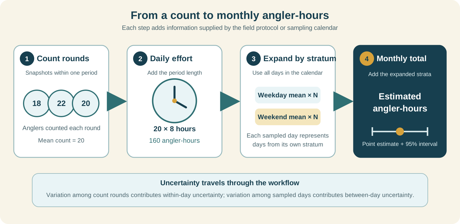
An instantaneous count answers a narrow question: how many anglers were present when the count was made? If 20 anglers are present at 10:15 a.m., the observation is 20 anglers. It is not 20 angler-hours and it is not the number of people who fished that day.

The count becomes an estimate of effort only after it is connected to time. If the count was randomized within an eight-hour fishing period, the simple period estimate is:

\[ \widehat{E}_{d} = I_d T_d, \]

where \(I_d\) is the instantaneous angler count and \(T_d\) is the length of the period in hours. A count of 20 anglers across an eight-hour period represents 160 angler-hours for that sampled day.

That multiplication depends on the field design. The eight hours must describe the period over which the count was randomized and for which the snapshot is intended to be representative. It should not be added later merely because the survey crew worked an eight-hour shift.

Multiple counts within a period add another step. They estimate the same stock of anglers at different moments, so they are averaged before multiplying by the period length. They are not summed as if each count found a new set of anglers. The longer treatment in Modern Creel Survey Analysis in R works through that within-day case.

The same logic carries those snapshots through to a monthly estimate:

Keep the full calendar and the sampled counts

This example covers June 1 through June 16. The full calendar defines ten weekdays and six weekend days. Counts were collected on five weekdays and three weekend days.

library(tidycreel)

dates <- seq(
  as.Date("2024-06-01"),
  as.Date("2024-06-16"),
  by = "day"
)

calendar <- data.frame(
  date = dates,
  day_type = ifelse(
    as.integer(format(dates, "%u")) >= 6L,
    "weekend",
    "weekday"
  )
)

sample_dates <- as.Date(c(
  "2024-06-03", "2024-06-05", "2024-06-07",
  "2024-06-11", "2024-06-13",
  "2024-06-01", "2024-06-08", "2024-06-15"
))

counts <- data.frame(
  date = sample_dates,
  day_type = c(rep("weekday", 5), rep("weekend", 3)),
  n_anglers = c(10, 12, 11, 14, 13, 20, 24, 22),
  period_hours = rep(8, 8)
)

The unsampled dates remain in calendar, even though they have no row in counts. That is the distinction introduced in the sampling-calendar post: the observations come from sampled days, while the calendar defines the population of days they can represent.

Weekday and weekend also remain separate. Weekend counts are higher in this example, and weekends were sampled at a different rate. Pooling the days before expansion would let the composition of the sample, rather than the sampling design, determine the result.

Let add_counts() establish the effort unit

The design connects the calendar to the count observations. The important argument here is period_length_col.

design <- creel_design(
  calendar,
  date = date,
  strata = day_type
) |>
  add_counts(
    counts,
    count_col = n_anglers,
    period_length_col = period_hours
  )

For each sampled date, add_counts() multiplies n_anglers by period_hours. It also records the resulting effort unit as angler-hours. That unit information matters later when an effort estimate is combined with a rate reported as fish per angler-hour.

If period_length_col is omitted, tidycreel 7.0.0 warns that an instantaneous count has been expanded without a period length. The resulting sum is not an angler-hour estimate. The warning is worth stopping for because no downstream formatting can repair a missing time basis.

This example uses one count per sampled day, which keeps the arithmetic visible. A survey with repeated counts should also supply count_time_col so tidycreel can average the within-period counts and retain their contribution to uncertainty.

Choose the population the estimate should represent

estimate_effort() makes the reporting target explicit. Three calls show the progression from observed sample days to the full calendar period.

sampled_effort <- estimate_effort(
  design,
  target = "sampled_days"
)

effort_by_stratum <- estimate_effort(
  design,
  by = day_type,
  target = "stratum_total"
)

period_effort <- estimate_effort(
  design,
  target = "period_total"
)

The checked 7.0.0 example produces:

Target	What it represents	Estimate (angler-hours)
sampled_days	The eight days with counts	1,008
stratum_total, weekday	All ten weekdays in the calendar	960
stratum_total, weekend	All six weekend days in the calendar	1,056
period_total	All 16 calendar days, summed across strata	2,016

The sampled-day total is the sum of the eight daily effort estimates. The stratum totals first estimate mean daily effort within weekday and weekend, then multiply those means by the number of calendar days in each stratum. The period total adds the two stratum totals.

In this small example, exactly half of the days were sampled, so the period total happens to be twice the sampled-day total. That shortcut will not usually work. Sampling fractions can differ among strata, period lengths can vary, and the full estimate must preserve those differences.

Read the uncertainty with the point estimate

Printing period_effort returns more than 2,016 angler-hours:

Method: Total
Variance: Taylor linearization
Confidence level: 95%
Effort target: period_total
Unit: angler-hours

estimate    se se_between se_within ci_lower ci_upper     n
    2016    56         56         0     1879     2153     8

The estimate is 2,016 angler-hours for the 16-day period. Its standard error is 56 angler-hours, and the 95% confidence interval runs from 1,879 to 2,153 angler-hours.

Here, se_between equals the total standard error because there is only one count on each sampled day. There is no replication within a day from which to estimate moment-to-moment variation, so se_within is zero. Zero does not mean angler abundance was perfectly stable within each day. It means this design did not measure that component.

With repeated count rounds, se_within can quantify within-day variation. Comparing it with se_between helps identify whether additional field effort would be better spent sampling more days or making more counts on days already selected.

Check what the estimate does and does not cover

Before reporting the result, I would ask:

• Does the calendar contain every day in the intended reporting period?
• Were the counts randomized within the periods named by period_length_col?
• Do the strata match the field sampling design rather than a grouping created after data collection?
• Are dates without counts known unsampled days, or are some missed visits or missing records?
• Does the output name the expected target and unit?
• Are the confidence interval and variance components reported with the point estimate?

The estimate cannot extend beyond its frame. If the count route omitted part of the lake, the result represents the covered area unless an additional, defensible spatial expansion is part of the design. Likewise, a June calendar cannot support a summer-season total that includes July and August.

This is why check_completeness(design) is a diagnostic rather than an automatic decision maker. It can identify calendar dates without counts. The survey record must tell us whether those dates were intentionally unsampled, missed in the field, or lost during data handling.

An instantaneous count is only a snapshot. The period length gives it a time unit, the calendar gives it a population of days, and stratification controls how sampled days represent that population. estimate_effort() keeps those pieces together and returns the uncertainty needed to interpret the total.

The next step is to combine effort with interview-based rates to estimate total catch, harvest, and release. That multiplication is meaningful only when the rate and effort describe compatible anglers, places, periods, and units.

Reference

• Pollock, K. H., C. M. Jones, and T. L. Brown. 1994. Angler survey methods and their applications in fisheries management. American Fisheries Society Special Publication 25, Bethesda, Maryland.